Computing geometry metadata
Contents
Computing geometry metadata
In this tutorial you will learn the basics of computing and analysing the observation geometry associated to input data products in PLF files. We will use GEOGEN and external tools for the visualisation of output Coverage GeoJSON files.
Prerequisites
We assume you have access to the GEOGEN Training JupyterHub platform and completed the previous tutorial Getting started. You can also follow this tutorial if you’re using GEOGEN on your local computer.
Steps
1. Choose a Product List File (PLF)
Browse the content of your data/plf directory and pick the PLF file your want to compute the geometry metadata for.
This directory is initially set to contain the same PLF files provided in the psa-geo package, which are curated and
used for testing prior to each GEOGEN operational release:
limb_sample_test.plf
mex_marsis_lst_test.plf
mex_sample_test.plf
mex_targetless_test.plf
mixed_pds_versions_test.plf
multiple_targets_test.plf
poles-antimeridian_crossing_test.plf
ros_sample_test.plf
smart1_sample_test.plf
start_stop_time_test.plf
tgo_sample_test.plf
2. Get a computation preview
In this example we are using mex_sample_test.plf as input PLF file:
$ geogen compute data/plf/mex_sample_test.plf
This command will return a list of valid data products grouped by coverage that have been loaded from the input PLF file. It displays assigned and derived product attributes for each product, and the directories in which output files are generated. For example:
[WARNING] Undefined or null input product_type: default <MEX/HRSC/RDR> product type definition used instead.
[WARNING] Undefined or null input product_type: default <MEX/HRSC/RDR> product type definition used instead.
[WARNING] Undefined or null input product_type: default <MEX/HRSC/RDR> product type definition used instead.
[WARNING] Undefined or null input product_type: default <MEX/HRSC/RDR> product type definition used instead.
[WARNING] Undefined or null input product_type: default <MEX/HRSC/RDR> product type definition used instead.
[WARNING] Undefined or null input product_type: default <MEX/HRSC/RDR> product type definition used instead.
[WARNING] Undefined or null input product_type: default <MEX/HRSC/RDR> product type definition used instead.
[WARNING] Undefined or null input product_type: default <MEX/HRSC/RDR> product type definition used instead.
[WARNING] Undefined or null input product_type: default <MEX/HRSC/RDR> product type definition used instead.
[WARNING] Undefined or null input product_type: default <MEX/HRSC/RDR> product type definition used instead.
[WARNING] Undefined or null input product_type: default <MEX/HRSC/RDR> product type definition used instead.
[WARNING] Undefined or null input product_type: default <MEX/HRSC/RDR> product type definition used instead.
8 coverage(s) loaded from PLF file:

#1 MARS_MEX_ASPERA-3_DATA has 3 observation(s):

   Product ID                    = IMA_AZ0720072732358C_ACCS01
   Product Type                  = DATA
   Target SPICE Name             = MARS
   Target SPICE Body-Fixed Frame = IAU_MARS
   GEOGEN Detector Type          = IN-SITU
   Detector SPICE Name           = MEX_ASPERA_IMA
   Detector SPICE ID             = -41151
   Detector SPICE Frame          = N/A
   Number of Data Records        = 4074
   Computation Time Steps        = 100
...

Output B3F directory     : /Users/nmanaud/workspace/geogen/data/b3f/mex_sample_test/
Output GeoJSON directory : /Users/nmanaud/workspace/geogen/data/geojson/mex_sample_test/

This was a computation preview. Use --no-preview option to run the computation.
2. Compute geometry
To run the actual computation, just add the --no-preview option:
$ geogen compute data/plf/mex_sample_test.plf --no-preview
You should see something like this:
[WARNING] Undefined or null input product_type: default <MEX/HRSC/RDR> product type definition used instead.
[WARNING] Undefined or null input product_type: default <MEX/HRSC/RDR> product type definition used instead.
[WARNING] Undefined or null input product_type: default <MEX/HRSC/RDR> product type definition used instead.
[WARNING] Undefined or null input product_type: default <MEX/HRSC/RDR> product type definition used instead.
[WARNING] Undefined or null input product_type: default <MEX/HRSC/RDR> product type definition used instead.
[WARNING] Undefined or null input product_type: default <MEX/HRSC/RDR> product type definition used instead.
[WARNING] Undefined or null input product_type: default <MEX/HRSC/RDR> product type definition used instead.
[WARNING] Undefined or null input product_type: default <MEX/HRSC/RDR> product type definition used instead.
[WARNING] Undefined or null input product_type: default <MEX/HRSC/RDR> product type definition used instead.
[WARNING] Undefined or null input product_type: default <MEX/HRSC/RDR> product type definition used instead.
[WARNING] Undefined or null input product_type: default <MEX/HRSC/RDR> product type definition used instead.
[WARNING] Undefined or null input product_type: default <MEX/HRSC/RDR> product type definition used instead.
Computing coverage geometry...
<Observation: product_id=IMA_AZ0720072732358C_ACCS01 valid=True>
<Observation: product_id=IMA_AZ0220072731630C_ACCS01 valid=True>
<Observation: product_id=IMA_AZ0020072640742C_ACCS01 valid=True>
Valid coverage observations: 3/3
Computing coverage footprints...
Writing coverage B3F file...
Writing coverage GeoJSON file...
Done.
...

DONE.
Output B3F directory     : /Users/nmanaud/workspace/geogen/data/b3f/mex_sample_test/
Output GeoJSON directory : /Users/nmanaud/workspace/geogen/data/geojson/mex_sample_test/
Output LOG file          : /Users/nmanaud/workspace/geogen/data/log/mex_sample_test_2022-02-28_17-33-34_515353.log
Should you see any WARNING or ERROR messages, please refer to Troubleshooting.
3. Inspect results
Look at the generated output files: directory structure, naming, content.
geojson/b3f/log/
Note
They are two different ways of opening a JSON file in the JupyterLab interface: open with Editor, or JSON (read-only, but useful to navigate the data structure).
We’ll see how to visualise GeoJSON files later.
4. Try other options
Using pre-configured digital model (DSK):
$ geogen compute psa_geo/data/plf/mex_sample_test.plf --dsk
It displays the list required DSK files, as defined in the config file:
Defined DSK files for target(s) in input PLF file:
- MARS: none
- PHOBOS: /Users/nmanaud/workspace/geogen/psa_geo/data/addendum/phobos_2014_09_22.bds

Loaded DSK files for target(s) in input PLF file:
None.
$ geogen compute psa_geo/data/plf/mex_sample_test.plf --dsk --no-preview
Splitting footprints geometry
By default the compute command doesn’t split output footprints geometry. Use the --split option:
geogen compute psa_geo/data/plf/mex_sample_test.plf --split --no-preview
Alternatively you can use the the split command:
geogen split data/geojson/mex_sample_test/phobos_mex_hrsc_rdr_dsk.json
Using different primary target

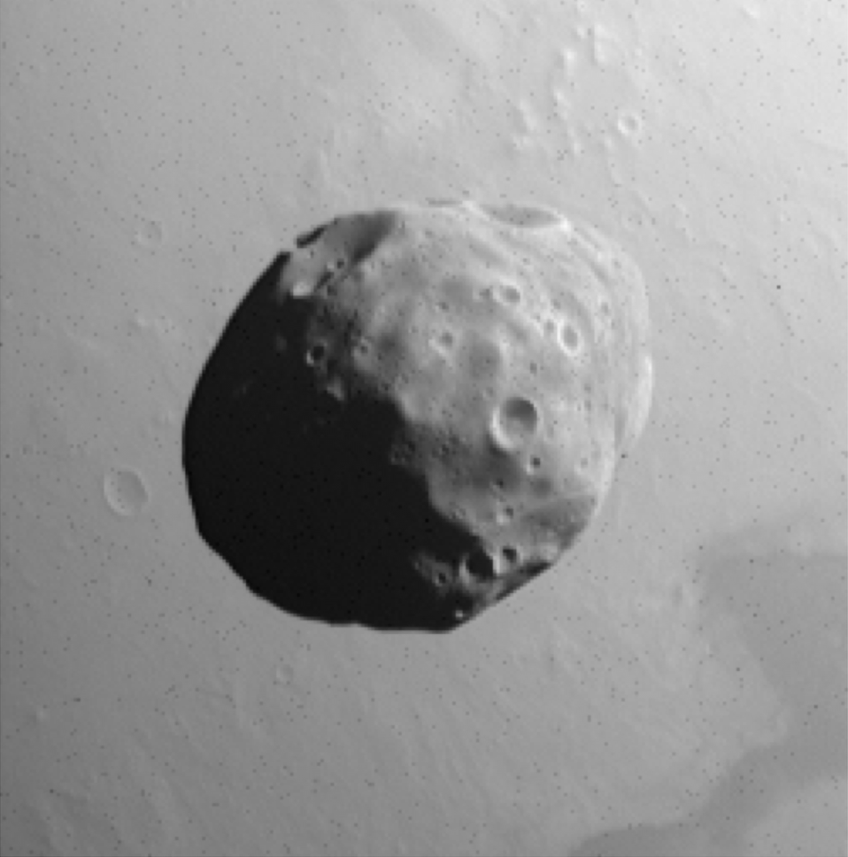
Mars Express HRSC Phobos observation (HD412_0005_SR2).
You can force a target to be different than the one assigned from the PLF file target_name propertie by using the
--forced-target option (see Target Assignment). Example:
$ geogen compute psa_geo/data/plf/mex_sample_test.plf --product-id=HD412_0005_SR2.IMG --forced-target=MARS

#1 PHOBOS_MEX_HRSC_RDR has 1 observation(s):

    Product ID                    = HD412_0005_SR2.IMG
    Product Type                  = RDR
    Target SPICE Name             = MARS
    Target SPICE Body-Fixed Frame = IAU_MARS
    GEOGEN Detector Type          = FRAME
    Detector SPICE Name           = MEX_HRSC_SRC
    Detector SPICE ID             = -41220
    Detector SPICE Frame          = MEX_HRSC_SRC
    Number of Data Records        = 1018
    Computation Time Steps        = 100

Output B3F directory     : /Users/nmanaud/workspace/geogen/data/b3f/mex_sample_test/
Output GeoJSON directory : /Users/nmanaud/workspace/geogen/data/geojson/mex_sample_test/
Attention
Each computation overwrites previous data files. Rename your output data files before running another computation with specific options or configuration if you want to preserve and compare different results.
5. Visualise geometry data
Visualising output Coverage GeoJSON files is key to validate GEOGEN computations for a given configuration. The following external tools can be used to visualise GeoJSON files:
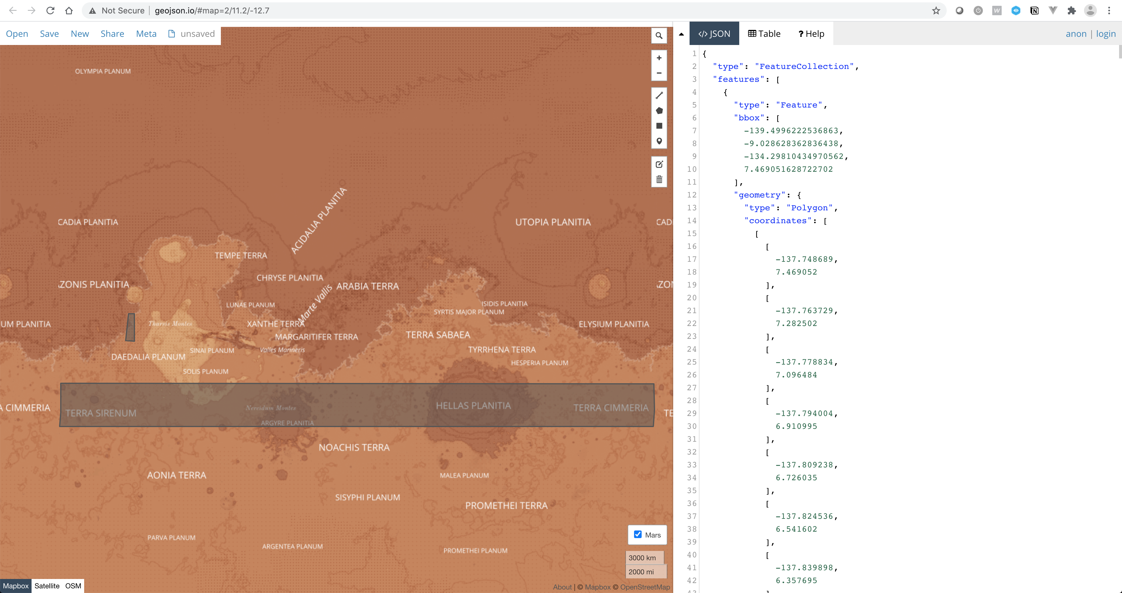
geojson.io
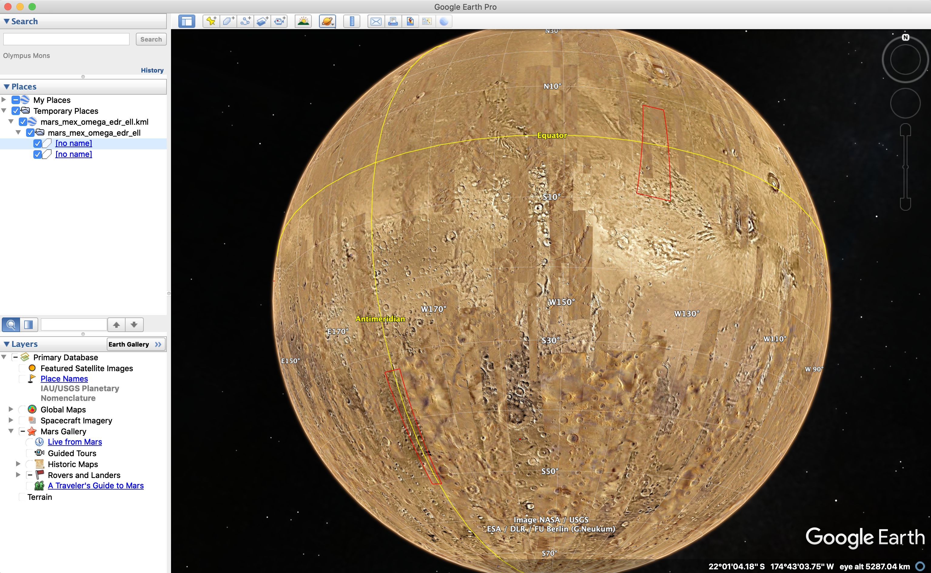
Google Earth
QGIS
JupyterLab
Use geojson.io to visualise and compare different computations.
geojson.io
geojson.io is a fast, simple web-based viewer and editor for geospatial data in GeoJSON format.
To use geojson.io (or any other applications running from your computer), we will to download all the files you want to visualise. This is cumbersome but that’s the best we can do for now.
Once on your computer, simple drag-n-drop your file in geojson.io.
Note
You can use this basemaps of Mars in geojson.io. In the menu, go to Meta>Add map layer, and copy and paste the following URL:
https://cartocdn-gusc.global.ssl.fastly.net/opmbuilder/api/v1/map/named/opm-mars-basemap-v0-2/all/{z}/{x}/{y}.png
Google Earth
Google Earth is great to visualise in 3D “unsplit” observations footprints. However it requires convert your GeoJSON file into KML, which can be easily done using the following GDAL command:
ogr2ogr -f KML mars_mex_omega_edr_ell.kml data/geojson/mex_sample_test/mars_mex_omega_edr_ell.json
QGIS
QGIS is great for further analysis of the data.
Here is a list USGS WMS URLs that you can use as basemap for a selection of target body:
https://planetarymaps.usgs.gov/cgi-bin/mapserv?map=/maps/mars/mars_simp_cyl.maphttps://planetarymaps.usgs.gov/cgi-bin/mapserv?map=/maps/mars/phobos_simp_cyl.maphttps://planetarymaps.usgs.gov/cgi-bin/mapserv?map=/maps/earth/moon_simp_cyl.maphttps://planetarymaps.usgs.gov/cgi-bin/mapserv?map=/maps/mercury/mercury_simp_cyl.maphttps://planetarymaps.usgs.gov/cgi-bin/mapserv?map=/maps/venus/venus_simp_cyl.map
JupyterLab
It would be the nicest solution to visualise and analyse GEOGEN output data. It would require further development.


